Estimate Error Rate of Services for Client of SSO • ssoestimate

For now: still work in progress

I have remade the SSO algorithm. It was wrong as it produced graphs where the client graph was more pronounced (had a higher peek) than the SSO graph, implying that the algorithm added information about the client, which is not possible.

The current algorithm is yet not satisfactory, which seems largely due to the application of the R density() function. I have possibly to make my own version of the density function or seek another approach, whereby I do not need Monte Carlo.

The story below is based on the previous algorithm, so it does not make much sense any more given the results as produced by the current algorithm. So the story below should be adapted.

Also to do is to move the most of the content of this README to a vignette for the ssoestimate package. But I did not succeeded so far in using vignettes on my computer system. Beats me why.

The current algorithm seems in the basics sound. And its results seems more intuitive appealing. One possible message to take away from the results is that in order to have precise results about the clients you have to combine information from both SSO and client. My impressions is that, if you want to be very specific about the client you either need very vast amounts of information solely from the SSO, or some info from the SSO + some info from the client. But, this is only a hunch, and needs more exploring.

Introduction

A shared Service Organisation, SSO, is an administrative entity that carries out financial transactions on behalf of a number of client organisations. The kind of transactions done by the SSO are the same for all clients.

The goal of the package ssoestimate is to estimate the error rate of transactions for each single client of the SSO. This is done by using a sample from all the transactions of the SSO as a proxy. Below we will sometimes refer to this sample as random sample 1. This assumes that the most efficient way to estimate this error rate is by means of sampling: it is not feasible, for example, to do an integral data-analyses of the transactions. The one big assumption that ssoestimate uses is that the set of transactions from the client is a random sample from all the transactions carried out by the SSO. Below we will sometimes refer to this sample as random sample 2.

Using this assumption makes it possible to efficiently estimate the error rate for all the clients of the SSO. For example suppose that

the SSO processed 100,000 transactions in total, for 10 clients
the SSO processed at least 1000 transactions per client
we want to establish with 95% confidence that the error rate for each client is at most 1%,

then we could use (expecting no errors in the samples) a sample of 300 transactions from each client, totaling 10x300 = 3000 transactions. Instead when using ssoestimate it suffices to draw only 350 transactions in total to conclude with 95% confidence that the error rate of each client is at most 1%. That is, for each client for which the assumption hold that the set of its transactions is a random sample of all the transactions carries out by the SSO. So by taking into account the smallest number of client transactions we get an upper limit estimation of the error rates of all those clients. Further, see the example below.

The package has two main functions:

SSO_estimate(), which makes the estimation, and
SSO_graph_plot(), which presents the estimation made by SSO_estimate().

Installation

You can install the development version of ssoestimate like so:

install.packages("devtools")
#> Installing package into '/tmp/Rtmp4jiirq/temp_libpathaeb568d080c'
#> (as 'lib' is unspecified)
# devtools::install_github("cfjdoedens/ssoestimate")
library(ssoestimate)

Example: visual presentation

This example shows that indeed 350 transactions (n_SSO = 350), which turn out to have no errors (k_SSO = 0), suffice to ascertain that a client which has 1000 transactions (N_client = 1000) has with 95% (cert = 0.95) certainty at most 1% errors (client max 0.010).

x <- SSO_estimate(k_SSO = 0, n_SSO = 350, N_client = 1000, S = 1000)
SSO_graph_plot(x)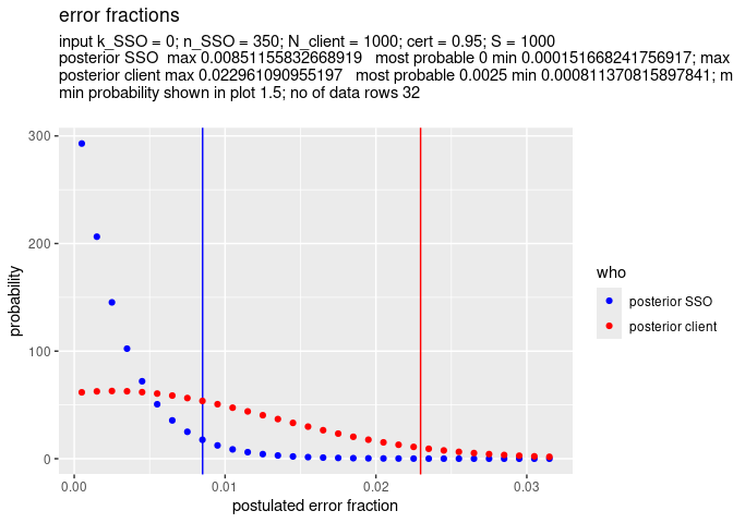

The estimated values for SSO max, SSO most probable, SSO min, and ditto for the client are rounded based on the value of S. The precision of the estimation is at most 1/(2*S). So, a higher value for S gives a better precision of the estimation. In this example the precision is at most 1/2000 = 0.0005.

Example: non visual presentation

We can show the result of the estimation carried out in the previous example also non visual.

SSO_graph_plot(x, visual = FALSE)
#> $prior_SSO_max
#> [1] 0.95
#> 
#> $prior_SSO_most_prob_p
#> [1] 0.5
#> 
#> $prior_SSO_min
#> [1] 0.05
#> 
#> $posterior_SSO_max
#> [1] 0.008511558
#> 
#> $posterior_SSO_most_prob_p
#> [1] 0
#> 
#> $posterior_SSO_min
#> [1] 0.0001516682
#> 
#> $prior_client_max
#> [1] 0.95
#> 
#> $prior_client_most_prob_p
#> [1] 0.5
#> 
#> $prior_client_min
#> [1] 0.05
#> 
#> $posterior_client_max
#> [1] 0.02296109
#> 
#> $posterior_client_most_prob_p
#> [1] 0.0025
#> 
#> $posterior_client_min
#> [1] 0.0008113708
#> 
#> $notes
#> NULL

The numbers shown in the non visual presentation are the raw results of the estimation; they differ slightly from those in the visual example, as the former numbers are not rounded, and the latter are rounded.

Example: use of priors

In the examples so far we have not illuminated that SSO_estimate() can also handle prior chance curves both for the SSO and for the client. In fact SSO_estimate() always uses priors both for the SSO and for the client. The default priors are the uniform priors, these assume that all error rates are equally likely. As an example we will now introduce a non uniform prior for SSO and for client.

Suppose we do a preliminary random sample of 10 transactions from the total mass of transactions handled by the SSO, no matter the client, and find that there are 0 errors. We can use this information as a prior for the mass of all SSO transactions. And suppose we do a preliminary random sample of 20 transactions done by the SSO specifically for the client, and we find 1 error. This will be our prior for the client transactions.

We decide to do a sample of 350 transactions from the total mass of SSO transactions. We find that there are no errors in this sample. In all there are 1037 transactions specifically for this client in the total mass of transactions of the SSO.

Now we are ready to call SSO_estimate() and SSO_graph_plot(). Default only the posteriors for SSO and client are shown by SSO_graph_plot(). But as the priors are not flat, it seems interesting enough to ask SSO_graph_plot() to show them in this example.


fun_prior_SSO <- function(p) {
  dbinom(0, 10, p)
}
fun_prior_client <- function(p) {
  dbinom(1, 20, p)
}

x <- SSO_estimate(fun_prior_SSO = fun_prior_SSO, k_SSO = 0, n_SSO = 350, fun_prior_client = fun_prior_client,  N_client = 1037, S = 1000)
SSO_graph_plot(x, plot_prior_SSO = TRUE,  plot_prior_client = TRUE)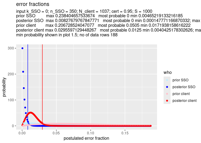

The most relevant, left side, of the graph is a bit compressed. So we zoom in a bit by setting min_prob = 10. This means that the graph will show only the part where the probability is at least 10 – see the left vertical axis.

SSO_graph_plot(x, plot_prior_SSO = TRUE, plot_prior_client = TRUE, min_prob = 10)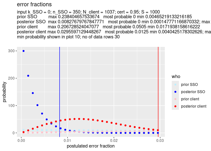

As you can see, the graph is more truncated at the right, making room to expand the left side of the graph.

Description of the algorithm behind SSO_estimate()

The algorithm of SSO_estimate() is based on the idea that we have two random samples of the same mass of SSO transactions. These two random samples are:

random sample 1, the random sample from the SSO as given by the parameters n_SSO and k_SSO, for respectively the number of transactions drawn, and the number of errors found in these transactions, and
random sample 2, the random sample from the SSO, being all the transactions from the client, and given by the parameter N_client, which has as value the number of client transactions done by the SSO for the client.

The algorithm of SSO_estimate() uses a grid which has two dimensions:

the possible error rates from 0 to 1 for the SSO transactions, and
the possible error rates from 0 to 1 for the client transactions.

Say, without loosing generality, that each row corresponds to a presumed value for the error rate of the client transactions, and that each column corresponds to a presumed value for a the error rate of the SSO transactions. In each grid location the probability of the presumed error rates for SSO and client is computed based on n_SSO, k_SSO and N_client; this is done by applying the binomial model both for the SSO transactions and for the client transactions. The probability of each presumed error rate of the client transactions is then computed as the marginal probability in the grid of that presumed error rate, so as the sum of the values in that row.

In the paragraph above we have abstracted away from the use of priors. In fact, the computation per grid location is augmented by multiplying each probability with the prior probability of the corresponding prior probability for the SSO, per column, and the corresponding prior probability for the client, per row.

All in all the code for the algorithm is not much more than a double loop, and some more lines.

Some questions and answers

What is the influence of the amount of client transactions on the closeness of the probability graphs of SSO error rate and client error rate, and why?

Answer: more client transactions brings the probability graph of the error rate of the client closer to the probability graph of the error rate of the SSO.

Explanation.

More client transactions means a bigger random sample (random sample 2) of the SSO transactions, meaning a more accurate estimate of the error rate of the transactions of the SSO.

The error rate of the SSO transactions is also estimated from the other random sample (random sample 1). Therefore when there are more client transactions the probability graph of the estimate of the error rate of the client transactions will become closer to the probability graph of the estimate of the error rate based on random sample 1.

Examples.

Below we see the effect of 10000 client transactions (N_client = 10000) versus 1000 client transactions (N_client = 1000)

x <- SSO_estimate(k_SSO = 0, n_SSO = 350, N_client = 10000, S = 1000)
SSO_graph_plot(x)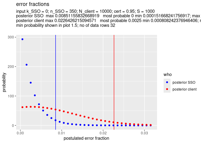

x <- SSO_estimate(k_SSO = 0, n_SSO = 350, N_client = 1000, S = 1000)
SSO_graph_plot(x)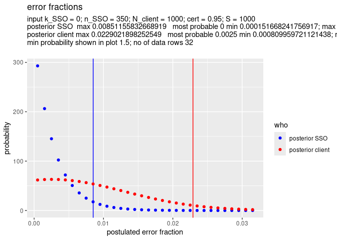

In both examples the maximum error fraction of the SSO is the same: 0.009, so 0.9 % error. This is as it should be, because the only difference between the parameters for the two examples is the value of N_client, and this value should not influence the estimate for the error rate of the SSO transactions.

However in the first example, the maximum error fraction for the cleint is In the first example, the difference between the maximum error fraction of SSO transaction client transactions (N_client = 20), instead of 1000 in the first example.

What is the influence of the amount of client transactions on the accuracy of the estimation of the error rate of the client, and why?

Answer: more client transactions makes the estimation of the error rate of the client transactions more accurate.

Explanation.

As explained directly above the more client transactions will bring the probability graphs of the error rate of client transactions and SSO transactions closer to each other. The ultimate knowledge we have of the error rate of the SSO transactions is given by the probability graph resulting from the sample of the SSO transactions (sample 1). This means that when the probability graph of the error rate of the client transactions comes closer to the probability graph of the the error rate of the SSO transactions, the accuracy of the estimation of the error rate of the client transactions improves.

To make this more clear. Assume sample 1 is very large, say, as big as all the transactions of the SSO transactions, then the accuracy of the estimation of the error rate of the client transaction will depend on the size of sample 2: a larger sample meaning a more accurate estimation.

In the description of the algorithm behind SSO_estimate() above, it is stated that the
computation of the probability for the presumed error rates of the client are based on the binomial model. Therefore, when the number of client transactions is small enough to make the binomial model less valid, this also diminishes the accuracy of the estimation of the error rate of the client.

What is the influence of the amount of SSO transactions on the estimation of the error rate of the SSO, and why?

Answer: The amount should be sufficient for the binomial model to give a valid estimation of the error rate of the SSO transactions.

Explanation.

SSO_estimate(), uses the binomial model for estimation of the error rate of the SSO transactions. For this model to give a valid estimation of the error rate, the SSO should have sufficiently many transactions to randomly sample from. Given a number of errors, the number of SSO transactions in itself does not change the estimation of the error rate of the SSO transactions. However when there are not enough SSO transactions, say less than thousand, the estimation becomes less valid. The assumption of sufficiently many SSO transactions that is sampled from, shows from the parameters of SSO_estimate(): there is no parameter for the number of SSO transactions. This because it is assumed there are sufficiently many, and given that there are sufficiently many it makes no difference how many precisely there are.

What is the influence of the amount of SSO transactions on the estimation of the error rate of the client, and why?

Answer: The amount should be sufficient for the binomial model, more makes no difference on the estimation of the error rate of the error rate of client transactions.

Explanation.

The estimation of the error rate of the client is based on the number of transactions of the client plus the estimation of the error rate of the SSO. When there are sufficiently many transactions for the SSO for the binomial model, and the number of transactions for the client is fixed, the estimation does not change when the number of transactions of the SSO increase, or decreases (while still be sufficiently many for the binomial model to hold).

What is the influence of the amount of client transactions, on the estimation of the error rate of the SSO, and why?

Answer: No influence

Explanation.

The estimation of the error rate of the SSO by SSO_estimate() is purely based on the number of samples, n_SSO, and the number of errors in that sample, k_SSO. So the number of client transactions plays no role.

Future extensions

Add monetary unit estimation

SSO_estimate() only works for the error fraction of the total number of transactions and not for the error fraction of the total monetary amount. In the future the function will be adapted to cater for both situations. For this it will be necessary to add the following parameters to SSO_estimate():

subject: Either transactions or monetary_amount.
total_amount_SSO: The total amount of money in the SSO transactions.
total_amount_client: The total amount of money in the client transactions.

Relax assumption that client transactions are a random sample of all transactions

The main supposition underlying SSO_estimate() is that the set of transactions from the client is a random sample from all the transactions carried out by the SSO. This is a strong assumption. Given that assumption we can place an upper limit on the estimate error rate for each client that satisfies the mentioned assumption of being a representative sample of all the transactions from the SSO, with only one random random sample from the SSO transactions.

As explained above, we can base the planned size of this one random sample on the expected error rate of the SSO and the number of transactions from the client with the lowest number of SSO transactions. The resulting estimation of the error rate is an upper limit for all clients which satisfy the assumption that their transactions from a random sample from the transactions of the SSO.

We can refine the estimation, and relax this assumption as follows. In practice some clients will have a more risky profile of transactions then other clients. What we could do is determine by means of data analysis, so not by drawing a sample, the risk profile of all the clients. And then find out which client has the highest level of risk for its transactions. We then draw a sample from the total mass of transactions of the SSO but skewed towards this highest level of risk. This way we have an upper estimate of the error rate for the total of transactions of the SSO, which, when used with SSO_estimate(), will translate in an upper estimate of the error rate of any client.